Mixture model target distribution tutorial
This tutorial demonstrates how to define mixture models for the LADD marginal distributions. The mixture models are combinations of two distributions of the same type, allowing for more diverse and multimodal definitions for LADD. Compared to using only a single distribution and parameters for the definition of a marginal LADD, the mixture model takes in two sets of input parameters and a weighting factor between the two distributions. The mixture model distributions for LADD can be used in all of the the methods: QSM direct, leaf cylinder library, and canopy hull methods.
Target LADD without mixture models
Let’s start by first defining a comparison foliage without mixture models. We use the same target distribution definitions as in the main_qsm_direct.m script.
% LADD relative height
TargetDistributions.dTypeLADDh = 'beta';
TargetDistributions.pLADDh = [6 2];
% LADD relative branch distance
TargetDistributions.dTypeLADDd = 'beta';
TargetDistributions.pLADDd = [3 1];
% LADD compass direction
TargetDistributions.dTypeLADDc = 'vonmises';
TargetDistributions.pLADDc = [pi/4 0.2];
% LOD inclination angle
TargetDistributions.dTypeLODinc = 'dewit';
TargetDistributions.fun_pLODinc = @(h,d,c) [1 2];
% LOD azimuth angle
TargetDistributions.dTypeLODaz = 'uniform';
TargetDistributions.fun_pLODaz = @(h,d,c) [];
% LSD
TargetDistributions.dTypeLSD = 'normal';
TargetDistributions.fun_pLSD = @(h,d,c) [0.014 0.00025^2];
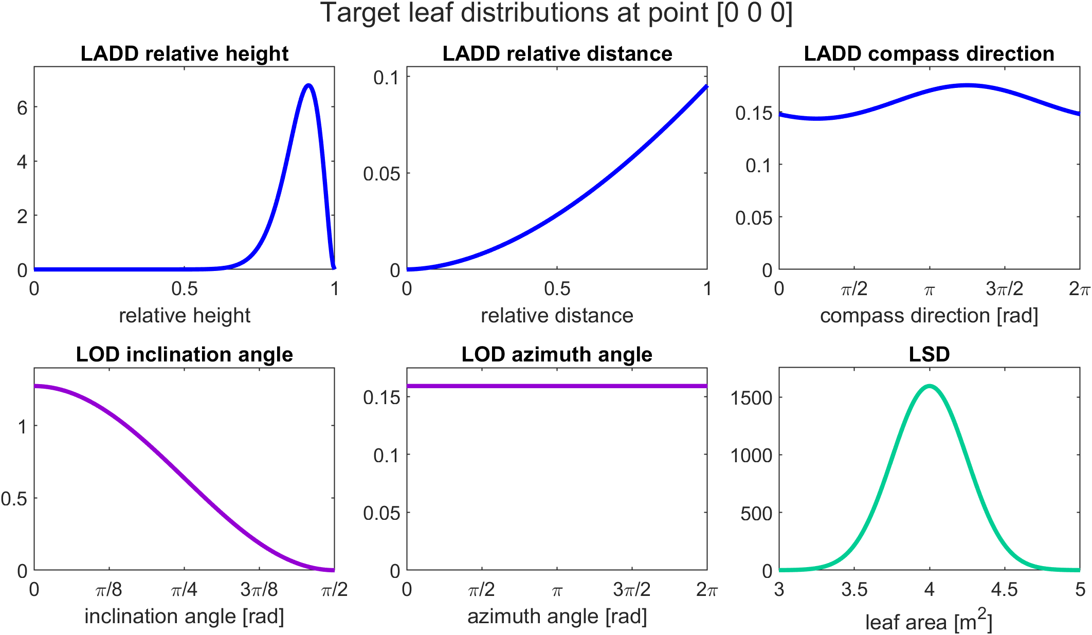
% Visualize the target distributions
visualize_target_distributions(TargetDistributions,[0 0 0]);
% Set the target leaf area
totalLeafArea = 60;
The visualization shows us the following distributions:
Target LADD with mixture models
Now let us define mixture models for the LADD marginal distributions. These can be achieved by adding the word “mixture” to the end of distribution type definition and providing the parameters of the second distribution and the weighting factor as extension to the parameter vector.
% LADD relative height
TargetDistributions.dTypeLADDh = 'betamixture';
TargetDistributions.pLADDh = [6 2 11 12 0.7];

% LADD relative branch distance
TargetDistributions.dTypeLADDd = 'betamixture';
TargetDistributions.pLADDd = [3 1 5 2 0.7];

% LADD compass direction
TargetDistributions.dTypeLADDc = 'vonmisesmixture';
TargetDistributions.pLADDc = [0.0 1.0 (4/5)*pi 1.0 0.75];

% LOD inclination angle
TargetDistributions.dTypeLODinc = 'dewit';
TargetDistributions.fun_pLODinc = @(h,d,c) [1 2];

% LOD azimuth angle
TargetDistributions.dTypeLODaz = 'uniform';
TargetDistributions.fun_pLODaz = @(h,d,c) [];

% LSD
TargetDistributions.dTypeLSD = 'normal';
TargetDistributions.fun_pLSD = @(h,d,c) [0.014 0.00025^2];

% Visualize the target distributions
visualize_target_distributions(TargetDistributions,[0 0 0]);

% Set the target leaf area
totalLeafArea = 80;
In this definition for heightwise LADD we use a mixture of beta distribution with the first one having parameters $\alpha = 6$ and $\beta = 2$, the second one having parameters $\alpha = 11$ and $\beta = 12$, and the weighting factor of $0.7$ on the first distribution (and thus weight $0.3$ on the second). The distancewise LADD uses a mixture of two beta distributions with the first one having parameters $\alpha = 3$ and $\beta = 1$, the second one having parameters $\alpha = 5$ and $\beta = 2$, and the weighting factor being $0.7$ on the first distribution (i.e. $0.3$ weight on the second). The compass direction LADD has a mixture of two von Mises distributions with the first one having parameters $\mu = 0$ and $\kappa = 1.0$, the second one having $\mu = \frac{4}{5} \pi$ and $\kappa = 1.0$, and weight $0.75$ on the first distribution (and $0.25$ on the second). Additionally, we increase the total leaf area from 60 to 80 square meters, since the mixture model LADD assigns leaf area also to the lower branches, which are mainly leafless in the basic tutorial example.
With these definitions, we get the following visualization:
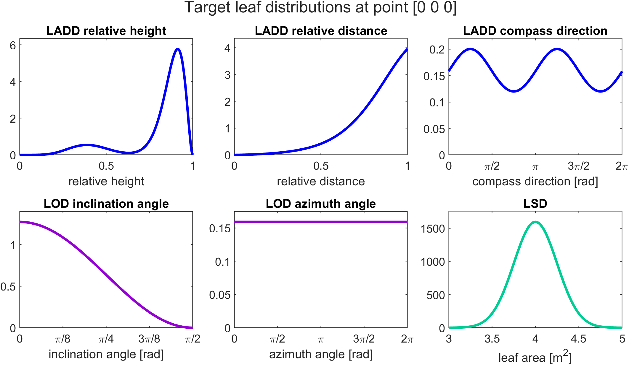
Here we can see the more detailed marginal LADD distributions (in blue) compared to the previous visualization.
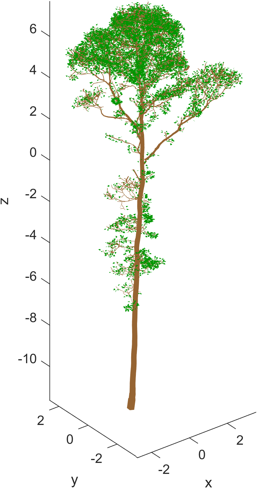
Resulting foliage
Below are figures of the foliage generated with each of the above definitions.
Without mixutre models:
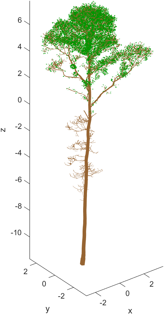
Using mixture models:
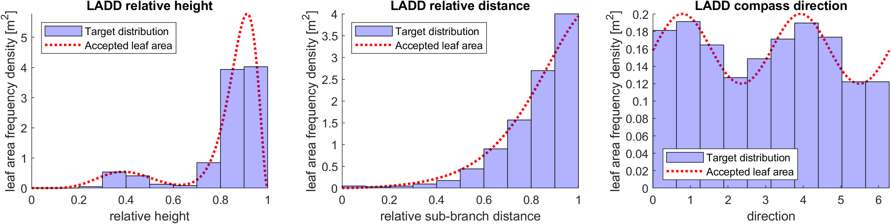
We can also plot the histograms of the LADD marginal distributions
Without mixture models:
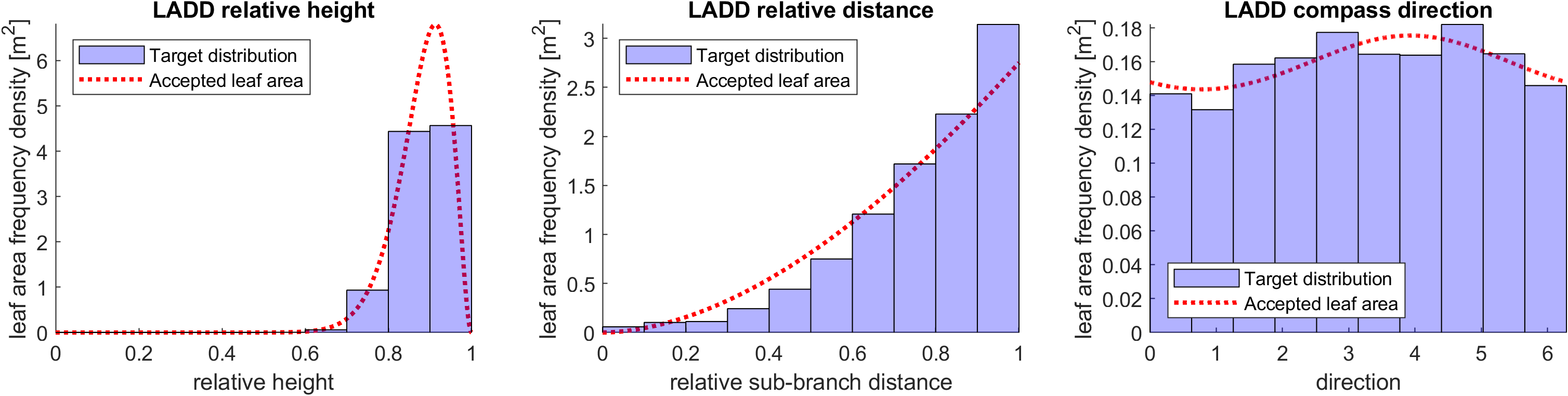
With mixture models: