Point cloud leaf position sampling tutorial
This tutorial demonstrates how to utilize the point cloud in leaf position sampling in the canopy hull method.
By default the canopy hull method generates an alpha shape around the tree point cloud and then samples the LADD within this shape to get the leaf positions. However, if the point cloud data is accurate, it makes sense to generate the leaves close to the point cloud points as these are realistic places for the leaves to be.
In addition, it might sometimes be useful to sample the leaf positions near the point cloud in the lower canopy, where the point cloud represents the branching sturcture more accurately, and use LADD in sampling for the upper part of the canopy, where the point cloud measurement is less accurate.
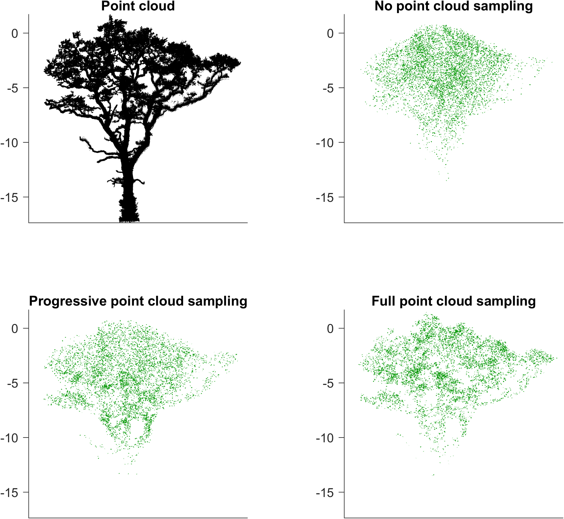
In this tutorial we demonstrate this feature by generating three different foliage on using the same point cloud as the basis for the canopy hull: The first one uses the default LADD sampling for leaf poisitions, the second one uses LADD sampling in the upper canopy and point cloud sampling in lower parts of the tree, and the third uses only point cloud in leaf position sampling.
Initialization
We start by clearing all workspace variables, closing all open figures and adding all the subdirectories to the MATLAB path.
% Clear all variables from the workspace and close all open figures
clear, close all

% Add the current directory and all the subdirectories to search path
addpath(genpath(pwd))
Leaf base geometry
The leaf base geometry is defined with vertice points and triangle vertice indices.
% Vertices of the leaf base geometry
LeafProperties.vertices = [0.0    0.0    0.0;
                           -0.04  0.02   0.0;
                           0.0    0.10   0.0;
                           0.04   0.02   0.0];

% Triangles of the leaf base geometry
LeafProperties.triangles = [1 2 3;
                            1 3 4];
Point cloud definition
In this example, the point cloud used as a basis for the foliage generation is from the Wytham woods dataset by Calders et al. 2022 (from DATA_QSM_OPT directory tree no. 8399). To do this we need to add the Wytham dataset folder to path and then import the .mat file to access the point cloud:
% Load point cloud from memory
addpath("<PATH_TO_WYTHAM_DATA>")
filename = "DATA_QSM_opt\wytham_winter_8399-0.2-0.22-3-0.045-0.0495-2-5-1-9.mat";
QSM = importdata(filename);
ptCloud = QSM.P;
To make sure the foliage is generated correctly, we need to translate the point cloud such that the stem center lies on z-axis, as this is the default assumption for the stem center. Here we assume the points spanning the bottom 1 meter of the point cloud to resemble the stem basis and translate their mean position to align with the z-axis.
% Center the point cloud to z-axis
stemBase = ptCloud((ptCloud(:,3) < min(ptCloud(:,3))+1),:);
baseMean = mean(stemBase,1);
ptCloud = ptCloud - [baseMean(1:2) 0];
Another option to ensure correct stem center would be to define the stem center coordinates manually and feed them as an additional parameter to the generate_foliage_canopy_hull function later on.
Leaf distributions
Next we define the target leaf distributions.
% LADD relative height
TargetDistributions.dTypeLADDh = 'beta';
TargetDistributions.pLADDh = [9 3.5];

% LADD relative distance from stem
TargetDistributions.dTypeLADDd = 'weibull';
TargetDistributions.pLADDd = [3.3 2.8];

% LADD compass direction
TargetDistributions.dTypeLADDc = 'vonmisesmixture';
TargetDistributions.pLADDc = [3/4*pi 2 7/4*pi 2 0.5];

% LOD inclination angle
TargetDistributions.dTypeLODinc = 'dewit';
TargetDistributions.fun_pLODinc = @(h,d,c) [-1 4];

% LOD azimuth angle
TargetDistributions.dTypeLODaz = 'uniform';
TargetDistributions.fun_pLODaz = @(h,d,c) [];

% LSD
TargetDistributions.dTypeLSD = 'normal';
TargetDistributions.fun_pLSD = @(h,d,c) [0.007 0.00025^2];
Target leaf area
The target leaf area for all three foliage is set to 50 square meters.
totalLeafArea = 50;
Generating foliage without point cloud sampling
The first foliage is generated completely based on sampling the defined leaf distributions (this is the default for canopy hull method)
[Leaves1,aShape] = generate_foliage_canopy_hull(ptCloud, ...
                                     TargetDistributions, ...
                                     LeafProperties, ...
                                     totalLeafArea);
At this point it is worthwile to check if the assumed stem center is properly inside the alphashape. It is ok if the assumed center line is slightly outside the shape in the very top or bottom of the point cloud, but if the centerline deviates from the shape in the middle of the point cloud, this can cause vertical gaps in the sampling of leaf start points.
f1 = figure(2); clf, hold on
plot(aShape,'FaceColor','m','FaceAlpha',0.2)
plot3([0 0],[0 0],[min(ptCloud(:,3)) max(ptCloud(:,3))],'c-', ...
      'LineWidth',3)
axis equal, axis off, view(45,0)
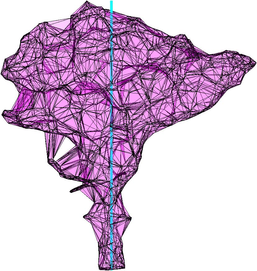
From the produced image we can see, that the stem center is inside the alpha shape (except for the very top, which is ok).
Generating foliage with progressive point cloud sampling
The second foliage is generated with progressive point cloud sampling: the lower parts of the canopy use the point cloud to inform the leaf start positions while the upper parts of the canopy use progressively more LADD. To achieve this, we need to feed an additional input to the generate_foliage_canopy_hull function known as “PCSamplingWeights”. This is a vector which defines the weighting for the use of point cloud sampling with respect to the relative height of the tree. The vector can have any number of elements and they contain the weights such that the first element corresponds to the lowers height stratum and the last element corresponds to the hightest. The height of the tree is automatically divided into equal height intervals based on the number of elements in the vector: a two-element vector splits the tree into two height strata whereas a eight-element vector creates eight different height strata.
In this example foliage, we decide to use only point cloud sampling for the lower half of the tree and starting from halfway we progressively emphasize LADD towards the top of the canopy. To do this, we define the first five elements of the weighting vector to have value 1 and starting from the sixth drop the weight to 0.8 and continue dropping the weight by 0.2 until the tenth element is 0. The code for doing this and generating the foliage is as follows:
% Define point cloud sampling weights
samplingWeights2 = [1 1 1 1 1 0.8 0.6 0.4 0.2 0];

% Generate foliage
[Leaves2,aShape] = generate_foliage_canopy_hull(ptCloud, ...
                                     TargetDistributions, ...
                                     LeafProperties, ...
                                     totalLeafArea, ...
                                     'PCSamplingWeights',samplingWeights2);
Generating foliage with full point cloud sampling
For the third foliage we want to use only point cloud sampling. Therefore, we define the point cloud sampling weight “vector” to consist of only one element with value 1. This assigns only one height stratum for the whole tree with full weight on point cloud sampling.
% Define point cloud sampling weight
samplingWeights3 = 1;

% Generate foliage
[Leaves3,aShape] = generate_foliage_canopy_hull(ptCloud, ...
                                     TargetDistributions, ...
                                     LeafProperties, ...
                                     totalLeafArea, ...
                                     'PCSamplingWeights',samplingWeights3);
Comparing the results
We can visualize the point cloud and all the resulting foliage with the following code:
f2 = figure(3); clf, hold on
tiledlayout(2,2)
s1 = nexttile(1);
plot3(ptCloud(:,1),ptCloud(:,2),ptCloud(:,3),'k.','MarkerSize',1)
axis equal, axis tight, view(45,0)
s1.XTick = []; s1.XTickLabel = []; s1.YTick = []; s1.YTickLabel = [];
title("Point cloud")
s2 = nexttile(2);
hLeaf1 = Leaves1.plot_leaves();
set(hLeaf1,'FaceColor',[0,150,0]./255,'EdgeColor','none');
axis equal, axis tight, view(45,0)
s2.XTick = []; s2.XTickLabel = []; s2.YTick = []; s2.YTickLabel = [];
title("No point cloud sampling")
s3 = nexttile(3);
hLeaf2 = Leaves2.plot_leaves();
set(hLeaf2,'FaceColor',[0,150,0]./255,'EdgeColor','none');
axis equal, axis tight, view(45,0)
s3.XTick = []; s3.XTickLabel = []; s3.YTick = []; s3.YTickLabel = [];
title("Progressive point cloud sampling")
s4 = nexttile(4);
hLeaf3 = Leaves3.plot_leaves();
set(hLeaf3,'FaceColor',[0,150,0]./255,'EdgeColor','none');
axis equal, axis tight, view(45,0)
s4.XTick = []; s4.XTickLabel = []; s4.YTick = []; s4.YTickLabel = [];
title("Full point cloud sampling")
linkaxes([s1 s2 s3 s4])
With this we can see the effect of the point cloud sampling in leaf positions.