Basic tutorial - QSM leaf cylinder library method
This tutorial goes over the example code main_qsm_leaf_cylinder_library.m provided along the GitHub repository, and demonstrates the very basic usage of the QSM leaf cylinder library method.
Initialization
The code starts by clearing the workspace (were the variables are stored), closing all open figures, and adding the paths to subdirectories required in this demo.
% Clear all variables from the workspace and close all open figures
clear, close all

% Add the current directory and all the subdirectories to search path
addpath(genpath(pwd))
Defining leaf base geometry
The leaf base geometry is defined by setting the vertice points of the geometry and indicating the triangles with respect to the vertices. These values are assigned to the LeafProperties struct.
% Vertices of the leaf base geometry
LeafProperties.vertices = [0.0    0.0    0.0;
                           -0.04  0.02   0.0;
                           0.0    0.10   0.0;
                           0.04   0.02   0.0];

% Triangles of the leaf base geometry
LeafProperties.triangles = [1 2 3;
                            1 3 4];
In the LeafProperties.vertices matrix each row corresponds to a singe vertice point and in the LeafProperties.triangles each row contains the row indices of vertices used for the triangles. These matrices define a leaf geometry based on two triangles which looks like this:
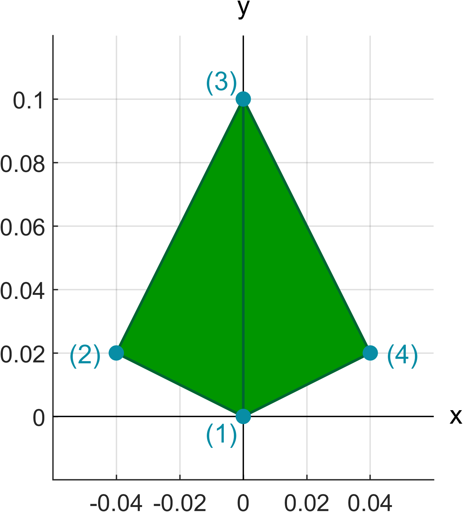
The absolute dimensions of the leaf base geometry are not important, since the base geometry is scaled to the correct size in the LSD sampling phase. Only the shape of the base geometry is preserved.
Setting petiole length limits
The leaf petioles are sampled unifromly from the interval defined to the LeafProperties struct:
LeafProperties.petioleLengthLimits = [0.08 0.10];
The units of the length limits are meters, so in this case the petioles are sampled between 8 and 10 centimeters.
Defining library LOD and LSD distribution types
For generatin a leaf cylinder library, we have to choose distribution type for the LOD inclination and azimuth distributions as well as for the LSD. This information is det into the LibraryVariables struct:
% Leaf orientation distribution types
LibraryDistributions.dTypeLODinc = 'dewit';
LibraryDistributions.dTypeLODaz  = 'vonmises';

% Leaf size distribution type
LibraryDistributions.dTypeLSD    = 'uniform';
In this example, the inclination angle marginal distribution is a generalized de Wit’s distribution, the azimuth angle marinal distribution is a von Mises distribution, and the LSD is a uniform distribution.
Defining the library nodes
The library consists of leaf cylinders with different attributes. These attributes are discretized and the discretization points are called nodes. So each node corresponds to some selection of cylinder and LOD & LSD attributes, and can contain one or multiple leaf cylinders with these attributes. When a leaf cylinder library is used to generate foliage on a QSM, for each cylinder of the QSM LeafGen finds the library node that corresponds closest to the attributes of the cylinder and picks one of the node’s leaf cylinders. The discretizations are defined to a struct named Nodes.
The leaf distribution attributes to discretize are:
- LOD inclination angle distribution parameters (two parameters)
- LOD azimuth angle distribution parameters (two parameters)
- LSD parameters (two parameters)
Since a library conists of single leaf cylinders, the LADD does not need to be defined at this point. It is only needed after the library generation when calculating leaf area budgets for a QSM.
The leaf distribution parameter discretizations are defined to the Nodes struct:
% Inclination angle distribution nodes
Nodes.pLODinc1 = [-1 0 1];
Nodes.pLODinc2 = [2 3 4];

% Azimuth angle distribution nodes
Nodes.pLODaz1   = [0 pi/2 pi 3*pi/2];
Nodes.pLODaz2   = [0.01 0.5];

% Leaf size distribution nodes
Nodes.pLSD1 = [0.010 0.012];
Nodes.pLSD2 = [0.014 0.016];
The cylinder attributes to discretize are:
- length
- radius
- inclination angle
- azimuth angle
- leaf area
These are also defined to Nodes struct:
Nodes.cylinderLength = [0.10 0.20];
Nodes.cylinderRadius = [0.01 0.05];
Nodes.cylinderInclinationAngle = [pi/4 3*pi/4];
Nodes.cylinderAzimuthAngle = [pi/4 3*pi/4 5*pi/4 7*pi/4];
Nodes.cylinderLeafArea = [0.2 0.5 0.8];
The number of discretization points in Nodes also defines the size of the leaf cylinder library. As the size of the library can grow exponentially when adding discratization points, the user should consider carefully for which attributes there should be more discretization points and which can do with less.
Leaf cylinder library generation
When we have the leaf base geometry, petiole lengths, LOD and LSD types, and discretization nodes, we can generate a leaf cylinder library with the function `generate_leaf_cylinder_library’.
LeafCylinderLibrary = generate_leaf_cylinder_library( ...
                          LibraryDistributions,Nodes,LeafProperties);
The function opens a parallel pool of computing cores to utilize parallel computation of the library cylinders. The progress of library generation is shown in a separate progress bar window.
The computation of a library this size takes quite a lot of computing resources. It is recommmended to use a supercomputer or a computer with large amount of processing cores to conduct the library generation.
Saving the leaf cylinder library
As generating a library requires a long computation, it is worth to save it for later use as a .mat file. This can be done with the command
save("NewLeafCyliderLibrary.mat",'-struct','LeafCylinderLibrary')
This creates a file called NewLeafCyliderLibrary.mat to the current working directory.
Defining the QSM
After generating a leaf cylinder library, we can use it to generate foliage on QSMs. The QSM used as a basis for leaf generation in this tutorial is the example QSM provided with the code repository of LeafGen. This is found in the example-data directory.
filename = "example-data/ExampleQSM.mat";
QSM = importdata(filename);
Defining target LADD and parameters for LOD and LSD
When generating foliage with the leaf cylinder library method, the LOD and LSD types are already chosen in the library generation phase. Therefore, for the leaf generation phase the user must define only the LADD marginal distributions and parameters as well as the LOD and LSD parameters.
The LADD marginal distributions are defined with a struct named TargetLADD:
% LADD relative height
TargetLADD.dTypeLADDh = 'beta';
TargetLADD.pLADDh = [6 2];

% LADD relative distance along sub-branch
TargetLADD.dTypeLADDd = 'beta';
TargetLADD.pLADDd = [3 1];

% LADD compass direction
TargetLADD.dTypeLADDc = 'vonmises';
TargetLADD.pLADDc = [pi/4 0.2];
The parameters for LOD and LSD are defined as functions of the structural variables of the QSM (relative height, relative branch distance, and compass direction). In this tutorial we define them to be stationary for the whole tree:
% LOD inclination angle
ParamFunctions.fun_pLODinc = @(h,d,c) [-1 4];

% LOD azimuth angle
ParamFunctions.fun_pLODaz = @(h,d,c) [pi 0.01];

% LSD
ParamFunctions.fun_pLSD = @(h,d,c) [0.012 0.014];
Since in this example our parameter functions have constant values for the whole tree, we can match their values exactly with the parameter discretization values we set for the nodes of the library above. If the parameter functions would have varying values in different parts of the tree, in leaf generation phase, the discretization node that corresponds most closely to the parameter values in that part is chosen when generating leaves on a cylinder there.
Setting target leaf area
The target leaf area is set in square meters to a variable named totalLeafArea:
totalLeafArea = 60;
The total leaf area can be essentially set to any positive value. In this case a total area of 60 square meters is chosen as the target. With the library method, the choice of target leaf area essentially has no effect on the speed of the foliage generation on the QSM. However, if the value is very large, the library cylinders might eventually lack leaves to fully reach the target.
A realistic choice for the target leaf area can be derived, for example, by multiplying some realistic leaf area index (LAI) value with the ground projected area of the tree crown.
Generating foliage on the QSM
Foliage generation on the QSM is conducted with the function transfrom_leaf_cylinders as follows:
[Leaves,QSMbc] = transform_leaf_cylinders(QSM,LeafCylinderLibrary, ...
                                          TargetLADD,ParamFunctions, ...
                                          totalLeafArea);
The first output Leaves contains a LeafModelTrianlge class object, which holds the transformation parameters of the generated leaves. The second output QSMbc contains the QSM as a QSMBCylindrical class object, which can be used to visualize and export the QSM.
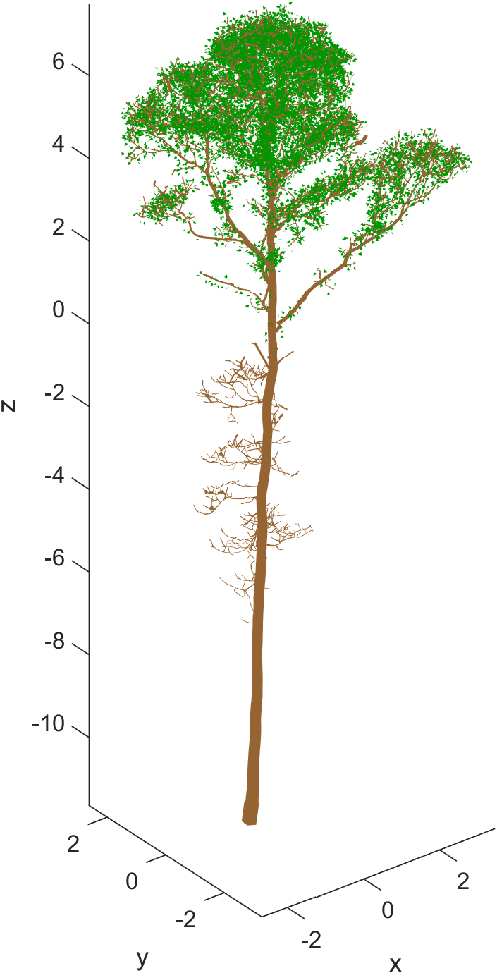
Visualizing the foliage in 3D
The generated foliage and the QSM can be visualized using class functions:
% Initialize figure
figure(1), clf, hold on

% Plot leaves
hLeaf = Leaves.plot_leaves();

% Set leaf color
set(hLeaf,'FaceColor',[0 150 0]./255,'EdgeColor','none');

% Plot QSM
hQSM = QSMbc.plot_model();

% Set bark color
set(hQSM,'FaceColor',[150 100 50]./255,'EdgeColor','none');

% Set figure properties
hold off;
axis equal;
xlabel('x')
ylabel('y')
zlabel('z')
This produces a 3D figure with green leaves and brown QSM.
Visualizing leaf distributions
The distributions of accepted leaves can be visualized with histograms.
LADD
The histograms of accepted leaf area with respect to each of the structural variables can be visualized alongside their target distributions with the following function calls:
plot_LADD_h_QSM(QSMbc,Leaves,TargetDistributions);
plot_LADD_d_QSM(QSMbc,Leaves,TargetDistributions);
plot_LADD_c_QSM(QSMbc,Leaves,TargetDistributions);
Here, again, h refers to relative height, d refers to relative branch distance, and c refers to compass direction.
LOD
The histograms of the inclination and azimuth angles of accepted leaves can be visualized with the following function calls:
plot_LOD_inc_QSM(QSMbc,Leaves);
plot_LOD_az_QSM(QSMbc,Leaves);
By default, these functions consider all leaves generated on the QSM, but they can be tuned to plot only specific intervals of the structural variables. In this tutorial the LOD for inclination and azimuth angles are stationary for the whole tree, so it makes sense to see the orientation histograms of all of the generated leaves.
LSD
The histogram of surface areas of accepted leaves can be visualized with the following function call:
plot_LSD_QSM(QSMbc,Leaves);
As with LOD, by default, this function considers all leaves generated on the QSM, but it can be tuned to plot only specific intervals of the structural variables. In this tutorial also the LSD is stationary for the whole tree, so it makes sense to see the leaf size histogram of the whole tree at once.
Exporting to OBJ files
The generated foliage and the QSM can be exported to Wavefront OBJ files using class functions.
% Precision parameter for export
precision = 5;

% Exporting to obj files
Leaves.export_geometry('OBJ',true,'leaves_export.obj',precision);
QSMbc.export('OBJ','qsm_export.obj','Precision',precision);
The precision parameter defines the number of digits used when writing the geometry to an OBJ file: higher values give more precise geometry but increase the file size, whereas small values reduce the file size but provide less accurate geometry.