Basic tutorial - QSM direct method
This tutorial goes over the example code main_qsm_direct.m provided along the GitHub repository, and demonstrates the very basic usage of the QSM direct method.
Initialization
The code starts by clearing the workspace (were the variables are stored), closing all open figures, and adding the paths to subdirectories required in this demo.
% Clear all variables from the workspace and close all open figures
clear, close all

% Add the current directory and all the subdirectories to search path
addpath(genpath(pwd))
Defining the QSM
The QSM used as a basis for leaf generation in this tutorial is the example QSM provided with the code repository of LeafGen. This is found in the example-data directory.
filename = "example-data/ExampleQSM.mat";
QSM = importdata(filename);
The example QSM is of the format given by TreeQSM, but the input QSM could also be a struct containing information of the QSM cylinders (see QSM direct method)
Defining leaf base geometry
The leaf base geometry is defined by setting the vertice points of the geometry and indicating the triangles with respect to the vertices. These values are assigned to the LeafProperties struct.
% Vertices of the leaf base geometry
LeafProperties.vertices = [0.0    0.0    0.0;
                           -0.04  0.02   0.0;
                           0.0    0.10   0.0;
                           0.04   0.02   0.0];

% Triangles of the leaf base geometry
LeafProperties.triangles = [1 2 3;
                            1 3 4];
In the LeafProperties.vertices matrix each row corresponds to a singe vertice point and in the LeafProperties.triangles each row contains the row indices of vertices used for the triangles. These matrices define a leaf geometry based on two triangles which looks like this:
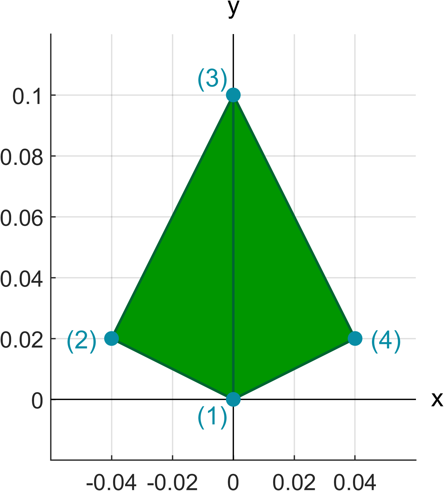
The absolute dimensions of the leaf base geometry are not important, since the base geometry is scaled to the correct size in the LSD sampling phase. Only the shape of the base geometry is preserved.
Setting petiole length limits
The leaf petioles are sampled unifromly from the interval defined to the LeafProperties struct:
LeafProperties.petioleLengthLimits = [0.08 0.10];
The units of the length limits are meters, so in this case the petioles are sampled between 8 and 10 centimeters.
Defining target leaf distributions
The target distribution types and parameters for LADD, LOD, and LSD are defined in the TargetDistributions struct.
The LADD marginal distribution types and parameters with respect to the structural variables are defined as:
% LADD relative height
TargetDistributions.dTypeLADDh = 'beta';
TargetDistributions.pLADDh = [6 2];

% LADD relative branch distance
TargetDistributions.dTypeLADDd = 'beta';
TargetDistributions.pLADDd = [3 1];

% LADD compass direction
TargetDistributions.dTypeLADDc = 'vonmises';
TargetDistributions.pLADDc = [pi/4 0.2];
Fields dTypeLADDh and pLADDh define the distribution type and parameters for the LADD marginal distribution on the relative height, in this case a beta distribution with parameters $\alpha$ = 6 and $\beta$ = 2. Similarly, dTypeLADDd and pLADDd define the relative branch distance marginal distribution as a beta distribution with the parameters $\alpha$ = 3 and $\beta$ = 1, and dTypeLADDc and pLADDc define the compass direction marginal distribution as a von Mises distribution with the mean direction of $\mu = \frac{\pi}{4}$ and the concentration parameter of $\kappa$ = 0.2.
The LOD marginal distribution types and parameters with respect to the inclination and azimuth angles of leaf normals are defined as:
% LOD inclination angle
TargetDistributions.dTypeLODinc = 'dewit';
TargetDistributions.fun_pLODinc = @(h,d,c) [1 2];

% LOD azimuth angle
TargetDistributions.dTypeLODaz = 'uniform';
TargetDistributions.fun_pLODaz = @(h,d,c) [];
The dTypeLODinc and fun_pLODinc fields define the distribution type for leaf inclination angle and the function for the distribution parameters, in this case a generalized de Wit’s distribution with parameters a = 1 and b = 2. The definition of distribution parameters, compared to LADD, is now done with a function, since the shape of LOD is allowed to change with respect to the structural variables. In this example, the parameters for inclination angle are set to be identical for the whole tree, so the field fun_pLODinc is set to be a handle for a constant function over all variable values. The dTypeLODaz and fun_pLODaz fields define the distribution type and parameters for the leaf azimuth angle, in this case a uniform distribution and thus an empty parameter function as no parameters are needed for uniform distribution on the azimuth angle (the distribution covers values from $0$ to $2\pi$ uniformly).
The LSD type and parameters, similarly to LOD, are defined as:
TargetDistributions.dTypeLSD = 'normal';
TargetDistributions.fun_pLSD = @(h,d,c) [0.014 0.00025^2];
The dTypeLSD and fun_pLSD fields define the distribution type and parameter function for the LSD, in this case a normal distribution with expected value of 140 square centimeters and a variance of 2.5$^2$ square centimeters.
The parameters of LOD inclination and azimuth angle distributions as well as LSD have to be given as function handles with three variables: relative height, relative branch distance, and compass direction. This holds even in the case they are constant or empty.
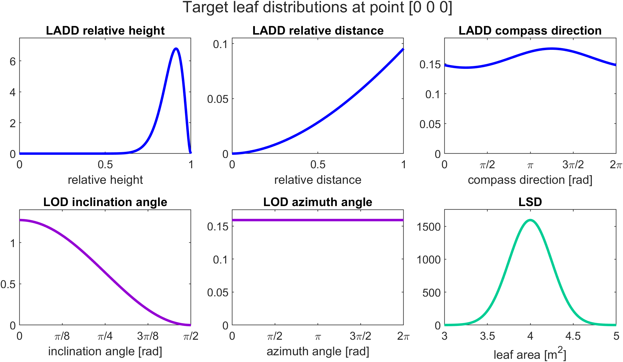
Before starting the leaf generation we can visualize the target distributions with the visualize_target_distributions function:
visualize_target_distributions(TargetDistributions,[0 0 0]);
The first input is the struct containing the distribution definitions and the second input is a vector for the structural variable coordinates of the point in which we want to visualize the distributions. In this case, all of our leaf distributions are stationary for the whole tree and do not vary depending on the structural variables, so we can put any point (in this case [0 0 0]) as the second input.
In the case of sructural-variable-dependent LOD or LSD, the shape of the distribution changes with respect to structural variable values. Therefore, when visualizing the target distributions, the user has to choose that for which part of the tree the distributions are visualized.
The visualization of the target distributions provides a figure showing the distributions we just defined above.
Setting target leaf area
The target leaf area is set in square meters to a variable named totalLeafArea:
totalLeafArea = 60;
The total leaf area can be essentially set to any positive value. In this case a total area of 60 square meters is chosen as the target. Larger values create larger foliage, which also increases the computational cost (mainly caused by the intersection prevention phase). If the value is too large the computation time can become very large as the overcrowding of leaves causes a lot of intersections. It is also possible that for too large total areas the target is not reached.
A realistic choice for the target leaf area can be derived, for example, by multiplying some realistic leaf area index (LAI) value with the ground projected area of the tree crown.
Generating foliage
The foliage is generated by calling the function generate_foliage_qsm_direct with the inputs defined above
[Leaves,QSMbc] = generate_foliage_qsm_direct(QSM,TargetDistributions, ...
                                             LeafProperties,totalLeafArea);
The first output Leaves contains a LeafModelTrianlge class object, which holds the transformation parameters of the generated leaves. The second output QSMbc contains the QSM as a QSMBCylindrical class object, which can be used to visualize and export the QSM.
Running this function can take some time if generating large or very dense foliage.
Visualizing the foliage in 3D
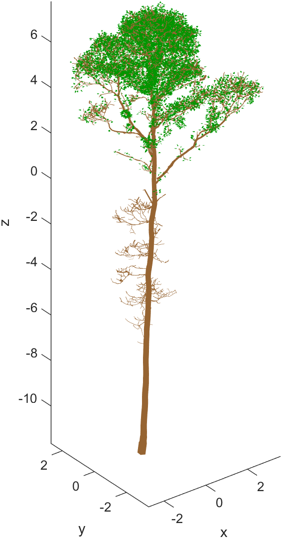
The generated foliage and the QSM can be visualized using class functions:
% Initialize figure
figure(1), clf, hold on

% Plot leaves
hLeaf = Leaves.plot_leaves();

% Set leaf color
set(hLeaf,'FaceColor',[0 150 0]./255,'EdgeColor','none');

% Plot QSM
hQSM = QSMbc.plot_model();

% Set bark color
set(hQSM,'FaceColor',[150 100 50]./255,'EdgeColor','none');

% Set figure properties
hold off;
axis equal;
xlabel('x')
ylabel('y')
zlabel('z')
This produces a 3D figure with green leaves and brown QSM.
Visualizing leaf distributions
The distributions of accepted leaves can be visualized with histograms.
LADD
The histograms of accepted leaf area with respect to each of the structural variables can be visualized alongside their target distributions with the following function calls:
plot_LADD_h_QSM(QSMbc,Leaves,TargetDistributions);
plot_LADD_d_QSM(QSMbc,Leaves,TargetDistributions);
plot_LADD_c_QSM(QSMbc,Leaves,TargetDistributions);
Here, again, h refers to relative height, d refers to relative branch distance, and c refers to compass direction.
LOD
The histograms of the inclination and azimuth angles of accepted leaves can be visualized with the following function calls:
plot_LOD_inc_QSM(QSMbc,Leaves);
plot_LOD_az_QSM(QSMbc,Leaves);
By default, these functions consider all leaves generated on the QSM, but they can be tuned to plot only specific intervals of the structural variables. In this tutorial the LOD for inclination and azimuth angles are stationary for the whole tree, so it makes sense to see the orientation histograms of all of the generated leaves.
LSD
The histogram of surface areas of accepted leaves can be visualized with the following function call:
plot_LSD_QSM(QSMbc,Leaves);
As with LOD, by default, this function considers all leaves generated on the QSM, but it can be tuned to plot only specific intervals of the structural variables. In this tutorial also the LSD is stationary for the whole tree, so it makes sense to see the leaf size histogram of the whole tree at once.
Exporting to OBJ files
The generated foliage and the QSM can be exported to Wavefront OBJ files using class functions.
% Precision parameter for export
precision = 5;

% Exporting to obj files
Leaves.export_geometry('OBJ',true,'leaves_export.obj',precision);
QSMbc.export('OBJ','qsm_export.obj','Precision',precision);
The precision parameter defines the number of digits used when writing the geometry to an OBJ file: higher values give more precise geometry but increase the file size, whereas small values reduce the file size but provide less accurate geometry.