Petiole direction and phyllotaxis tutorial
This tutorial demonstrates how to define petiole direction distributions or phyllotaxis patterns on QSM based foliage.
By default, within a single QSM cylinder, the start positions of leaf petioles are chosen randomly. The petiole direction distribution allows for weighing certain directions to generate more species specific behaviour, for instance, by emphasizing leaf origination to the side directions of the branch. On the other hand, if there is a spieces-specific pattern for the leaf positions, i.e., phyllotaxis pattern, this can be encoded to the foliage generation as well.
In this tutorial we first generate example cylinders showing the (I) unifrom leaf positioning, (II) the effect of petiole direction distribution, and (III) a cylinder with a phyllotaxis pattern. After demonstrating the effect on a local level we generate foliage on a full QSM based on all three approaches.
Initialization
The code starts by clearing the workspace (were the variables are stored), closing all open figures, and adding the paths to subdirectories.
% Clear all variables from the workspace and close all open figures
clear, close all

% Add the current directory and all the subdirectories to search path
addpath(genpath(pwd))
Leaf base geometry and petiole lengths
The leaf base geometry is defined with two triangles
% Vertices of the leaf base geometry
LeafProperties.vertices = [0.0    0.0    0.0;
                           -0.04  0.02   0.0;
                           0.0    0.10   0.0;
                           0.04   0.02   0.0];

% Triangles of the leaf base geometry
LeafProperties.triangles = [1 2 3;
                            1 3 4];
The petiole sampling interval is set between 4 cm and 6 cm
LeafProperties.petioleLengthLimits = [0.04 0.06];
LOD and LSD
To generate example leaf cylinders for the three cases, we need to define distributions for the leaf orientation and leaf size (i.e. LOD and LSD). For the leaf inclination angle we use a beta distribution highly skewed towards zero to generate horizontally oriented leaves to better visualize the effect of petiole direction and phyllotaxis. The leaf azimuth angle and leaf size distributions are set to uniform.
% LOD inclination angle
TargetDistributions.dTypeLODinc = 'beta';
TargetDistributions.fun_pLODinc = @(h,d,c) [1 10];

% LOD azimuth angle
TargetDistributions.dTypeLODaz = 'uniform';
TargetDistributions.fun_pLODaz = @(h,d,c) [];

% LSD
TargetDistributions.dTypeLSD = 'uniform';
TargetDistributions.fun_pLSD = @(h,d,c) [0.004 0.005];
For the cylinder demonstrations, we set the target leaf area to be 0.2 $\text{m}^2$ for a single cylinder.
leafArea = 0.2;
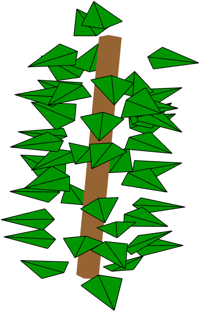
Uniform sampling on a cylinder
First we demonstrate the default approach of LeafGen in determining the petiole positioning on a single cylinder: the uniform positioning. To generate single leaf cylinders we use the function single_leaf_cylinder, which as a minimum input requires the TargetDistributions struct containing LOD and LSD info, LeafProperties struct containing the base geometry and petiole length limits, and the leafArea value containing the target leaf area.
% Generate leaves on a cylinder
[Leaves1,QSMbc1] = single_leaf_cylinder(TargetDistributions, ...
                       LeafProperties, leafArea);

% Plot the leaves
f1 = figure(1); clf, hold on
hQSM1 = QSMbc1.plot_model();
set(hQSM1,'FaceColor',[150 100 50]./255,'EdgeColor','none');
hLeaf1 = Leaves1.plot_leaves();
set(hLeaf1,'FaceColor',[0 150 0]./255,'EdgeColor','k');
axis equal, axis off, hold off
This generates the foliage on a cylinder and displays a visualization:
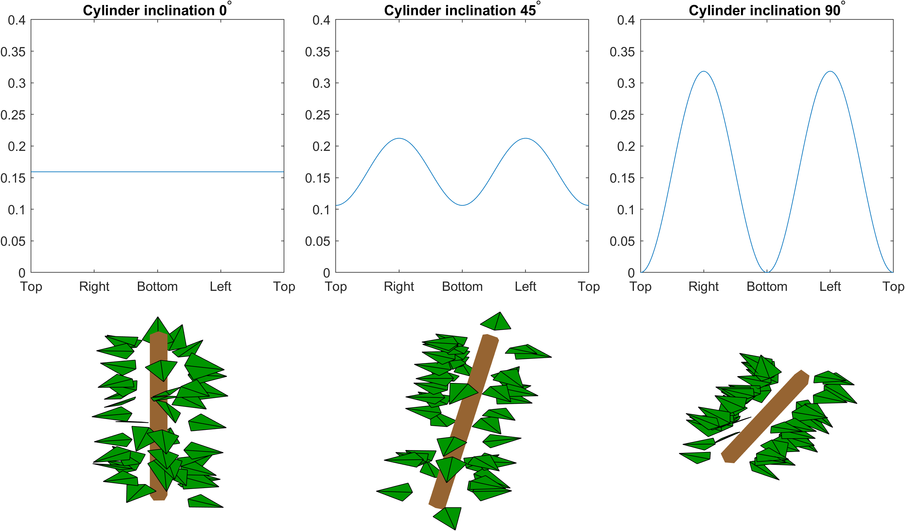
Petiole direction distribution on a cylinder
Now we determine a distribution for the petiole directions. This is done by defining a function handle which contains the distribution function for the petiole directions such that:
1) The direction is defined as an angular value between $0$ and $2\pi$ such that $0$ angle is the upmost radial direction on the cylinder. The angle increases following the right hand rule with respect to cylinder axis direction. At angle value $2\pi$ the direction meets the upmost radial direction of the angle $0$. If the cylinder axis is completely vertical and there is no upmost radial direction, the $0$ angle corresponds to the north direction. 2) The distribution function is defined for five variables, from which one is the actual variable of the distribution and other four are parameters of the cylinder: - The petiole direction angle (the actual variable) - The length of the cylinder - The radius of the cylinder - The inclination angle of the cylinder - The azimuth angle of the cylinder This way the petiole direction distribution can be set dependent on the cylinder attributes.
In this example we define a petiole direction distribution that is dependent only on the inclination angle of the cylinder:
pet_dir_fun = @(x,len,rad,inc,az) 1 - (1-2*inc/pi)*cos(x).^2;
Here x,len,rad,inc, and az are the petiole direction angle, cylinder length, cylinder radius, cylinder inclination angle, and cylinder azimuth angle, respectively. This distribution function gives uniform sampling of petiole direction for vertical cylinders, and gradually starts empasizing the sides of the cylinder more and more as the cylinder inclination angle increases.
Let’s generate three cylinders with inclination angles $0$, $\pi/4$ and $\pi/2$, that is, a vertical cylinder, a cylinder with 45 degree inclination, and a horizontal cylinder. The below code visualizes the petiole direction distribution for each of the cylinders, generates the foliage on them, and visualizes the cylinders with the generated leaves:
% Visualization of the distribution on different cylinder inclination
% angles
xx = 0:0.01:2*pi;
f2 = figure(2); clf, tiledlayout(2,3,"TileSpacing","tight")
axLimits = [0 2*pi 0 0.4];
yy1 = pet_dir_fun(xx,0,0,0,0); yy1 = yy1/trapz(xx,yy1);
nexttile(1), plot(xx,yy1), axis(axLimits), axis square
title('Cylinder inclination 0^{\circ}')
xticks([0 pi/2 pi 3*pi/2 2*pi])
xticklabels({'Top','Right','Bottom','Left','Top'})
yy2 = pet_dir_fun(xx,0,0,pi/4,0); yy2 = yy2/trapz(xx,yy2);
nexttile(2), plot(xx,yy2), axis(axLimits), axis square
title('Cylinder inclination 45^{\circ}')
xticks([0 pi/2 pi 3*pi/2 2*pi])
xticklabels({'Top','Right','Bottom','Left','Top'})
yy3 = pet_dir_fun(xx,0,0,pi/2,0); yy3 = yy3/trapz(xx,yy3);
nexttile(3), plot(xx,yy3), axis(axLimits), axis square
title('Cylinder inclination 90^{\circ}')
xticks([0 pi/2 pi 3*pi/2 2*pi])
xticklabels({'Top','Right','Bottom','Left','Top'})

% Generate leaves on three cylinders of different inclination angles
CylProperties.cylinderLength = 0.5;
CylProperties.cylinderRadius = 0.025;
CylProperties.cylinderAzimuthAngle   = -pi/4;
% Inclination angle 0 (vertical cylinder)
CylProperties.cylinderInclinationAngle = 0;
[Leaves2a,QSMbc2a] = single_leaf_cylinder(TargetDistributions, ...
                       LeafProperties, leafArea, ...
                       'PetioleDirectionDistribution', pet_dir_fun, ...
                       'CylinderProperties', CylProperties);
% Inclination angle pi/4 = 45 degrees
CylProperties.cylinderInclinationAngle = pi/4;
[Leaves2b,QSMbc2b] = single_leaf_cylinder(TargetDistributions, ...
                       LeafProperties, leafArea, ...
                       'PetioleDirectionDistribution', pet_dir_fun, ...
                       'CylinderProperties', CylProperties);
% Inclination angle pi/2 = 90 degrees (horizontal cylinder)
CylProperties.cylinderInclinationAngle = pi/2;
[Leaves2c,QSMbc2c] = single_leaf_cylinder(TargetDistributions, ...
                       LeafProperties, leafArea, ...
                       'PetioleDirectionDistribution', pet_dir_fun, ...
                       'CylinderProperties', CylProperties);

% Plot the leaves
nexttile(4), hold on
hQSM2a = QSMbc2a.plot_model();
set(hQSM2a,'FaceColor',[150 100 50]./255,'EdgeColor','none');
hLeaf2a = Leaves2a.plot_leaves();
set(hLeaf2a,'FaceColor',[0 150 0]./255,'EdgeColor','k');
view(-20,30), axis equal, axis off, hold off
nexttile(5), hold on
hQSM2b = QSMbc2b.plot_model();
set(hQSM2b,'FaceColor',[150 100 50]./255,'EdgeColor','none');
hLeaf2b = Leaves2b.plot_leaves();
set(hLeaf2b,'FaceColor',[0 150 0]./255,'EdgeColor','k');
view(-20,30), axis equal, axis off, hold off
nexttile(6), hold on
hQSM2c = QSMbc2c.plot_model();
set(hQSM2c,'FaceColor',[150 100 50]./255,'EdgeColor','none');
hLeaf2c = Leaves2c.plot_leaves();
set(hLeaf2c,'FaceColor',[0 150 0]./255,'EdgeColor','k');
view(-20,30), axis equal, axis off, hold off
This creates the following visualization:
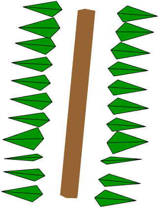
Phyllotaxis pattern on a cylinder
Lastly, we determine a phyllotaxis pattern of leaves. This is done by defining a struct which contains the parameters for the pattern. The pattern is defined in terms of nodes, which are points along the branch where a petiole or petioles of leaves originate.
There are five parameters to define:
1) nNodeLeaves: The number of leaves originating from a single node 2) petioleSeparationAngle: The angle between the petioles within a single node 3) nodeDistance: The distance between successive nodes on a branch 4) nodeRotation: The rotation of the petiole pattern between successive nodes 5) initialRadialAngle: The radial angle of the first leaf petiole on the first node ($0$ and $2\pi$ correspond to the upmost radial direction). This parameter sets the orientation of the pattern.
In LeafGen, the petiole direction is by default the same as the direction where the leaf is pointing and the petiole and the leaf form a rigid unit. However, to accomplish a phyllotaxis pattern in addition to following a user-defined LOD, the petioles in a phyllotaxis pattern are always directed in the radial direction of the cylinder (i.e. point outwards from the cylinder center) and the leaf tip direction can deviate from this.
We define these parameters on a struct called Phyllotaxis:
Phyllotaxis.nNodeLeaves  = 2;
Phyllotaxis.petioleSeparationAngle = pi;
Phyllotaxis.nodeDistance = 0.05;
Phyllotaxis.nodeRotation = 0;
Phyllotaxis.initialRadialAngle = pi/2;
In this pattern we have 2 leaves per node, the separation angle of their petioles is $\pi$ (180 degrees), distance between nodes is 5 cm, there is no rotation between nodes (angle of rotation defined 0 here), and the starting angle of the first leaf of first node is $\pi/2$ (90 degrees). These define a pattern where on each node there are two leaves with petioles pointing to both sides of the cylinder. To visualize this we generate the phyllotaxis pattern on a cylinder:
% Generate leaves on a cylinder
[Leaves3,QSMbc3] = single_leaf_cylinder(TargetDistributions, ...
                       LeafProperties, leafArea, ...
                       'Phyllotaxis', Phyllotaxis);

% Plot leaves
f3 = figure(3); clf, hold on
hQSM3 = QSMbc3.plot_model();
set(hQSM3,'FaceColor',[150 100 50]./255,'EdgeColor','none');
hLeaf3 = Leaves3.plot_leaves();
set(hLeaf3,'FaceColor',[0 150 0]./255,'EdgeColor','k');
axis equal, axis off, hold off
This creates the following visualization:
Applying to QSM direct method
Next we apply the above three approaches to foliage generation on a QSM. First we need to define some LADD to the TargetDistributions struct and set the QSM we want the leaves to be generated on.
% LADD relative height
TargetDistributions.dTypeLADDh = 'beta';
TargetDistributions.pLADDh = [6 2];

% LADD relative branch distance
TargetDistributions.dTypeLADDd = 'beta';
TargetDistributions.pLADDd = [3 1];

% LADD compass direction
TargetDistributions.dTypeLADDc = 'vonmises';
TargetDistributions.pLADDc = [pi/4 0.2];

% Load QSM
filename = "example-data/ExampleQSM.mat";
QSM = importdata(filename);
The we define the target leaf area and generate three different foliage: one with uniform position sampling within cylinders, one with the above petiole direction distribution, and one with the above phyllotaxis pattern:
% Define target leaf area
totalLeafArea = 60;

% Uniform leaf direction sampling
[Leaves4,QSMbc4] = generate_foliage_qsm_direct(QSM, ...
                       TargetDistributions, ...
                       LeafProperties, ...
                       totalLeafArea);

% Petiole direction distribution
[Leaves5,QSMbc5] = generate_foliage_qsm_direct(QSM, ...
                       TargetDistributions, ...
                       LeafProperties, ...
                       totalLeafArea, ...
                       'PetioleDirectionDistribution', pet_dir_fun);

% Phyllotaxis
[Leaves6,QSMbc6] = generate_foliage_qsm_direct(QSM, ...
                       TargetDistributions, ...
                       LeafProperties, ...
                       totalLeafArea, ...
                       'Phyllotaxis', Phyllotaxis);
The resulting foliage can be visualized with
f4 = figure(4); clf, hold on, tiledlayout(1,3)
nexttile(1)
hQSM4 = QSMbc4.plot_model();
set(hQSM4,'FaceColor',[150 100 50]./255,'EdgeColor','none');
hLeaf4 = Leaves4.plot_leaves();
set(hLeaf4,'FaceColor',[0 150 0]./255,'EdgeColor','none');
axis equal, axis off
nexttile(2)
hQSM5 = QSMbc5.plot_model();
set(hQSM5,'FaceColor',[150 100 50]./255,'EdgeColor','none');
hLeaf5 = Leaves5.plot_leaves();
set(hLeaf5,'FaceColor',[0 150 0]./255,'EdgeColor','none');
axis equal, axis off
nexttile(3)
hQSM6 = QSMbc6.plot_model();
set(hQSM6,'FaceColor',[150 100 50]./255,'EdgeColor','none');
hLeaf6 = Leaves6.plot_leaves();
set(hLeaf6,'FaceColor',[0 150 0]./255,'EdgeColor','none');
axis equal, axis off
This provides us with the following visualization.
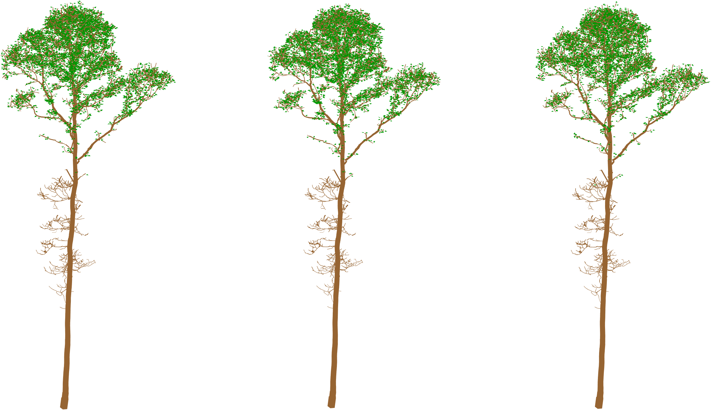
When using a phyllotaxis pattern, sometimes the target leaf area cannot be reached as the pattern limits the amount of leaf area that can be generated on a cylinder. Thus, if the LADD determines a large amount of leaf area for a single cylinder, this cannot be realized and the target is not reached. In the above example, the tree with the phyllotaxis pattern reached total leaf area of only 46 square meters instead of the target of 60 square meters.